Main Features of Combine
This exercise is designed to recreate the main workflow needed to perform a statistical analysis with Combine. It will start assuming you already prepared your inputs (shapes, yields, and systematic uncertainties) and will proceed step by step to perform validation test of your setup and produce some standard results. For more detailed procedure you can always find detailed informations in the Combine manual and in the Long exercise tutorial.
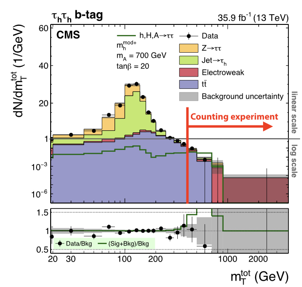
As for the Long exercise, we will work with a simplified version of a real analysis, that nonetheless will have many features of the full analysis. The analysis is a search for an additional heavy neutral Higgs boson decaying to tau lepton pairs. Such a signature is predicted in many extensions of the standard model, in particular the minimal supersymmetric standard model (MSSM). You can read about the analysis in the paper here. The statistical inference makes use of a variable called the total transverse mass (\(M_{\mathrm{T}}^{\mathrm{tot}}\)) that provides good discrimination between the resonant high-mass signal and the main backgrounds, which have a falling distribution in this high-mass region. The events selected in the analysis are split into several categories which target the main di-tau final states as well as the two main production modes: gluon-fusion (ggH) and b-jet associated production (bbH). One example is given below for the fully-hadronic final state in the b-tag category which targets the bbH signal:
Background
You can find a presentation with some more background on likelihoods and extracting confidence intervals here. A presentation that discusses limit setting in more detail can be found here. If you are not yet familiar with these concepts, or would like to refresh your memory, we recommend that you have a look at these presentations before you start with the exercise.
Getting started
To get started, you should have a working setup of Combine, please follow the instructions from the home page. Make sure to use the latest recommended release.
Now we will move to the working directory for this tutorial, which contains all the inputs needed to run the exercises below:
cd $CMSSW_BASE/src/HiggsAnalysis/CombinedLimit/data/tutorials/longexercise/
Part 1: Setting up the datacard and the workspace
Topics covered in this section:
- A: Setting up the datacard and the workspace
- B: MC statistical uncertainties
- C: Introducing control regions
[!TIP] To prepare the datacards you will need to collect all your inputs. This means having already selected, categorised, and analysed your data and MC, and having a settled strategy for at least the main background sources, so you are already well advanced in your analysis. Nevertheless, since without datacards you don't know yet how your results behave, we recommend to have this section ready during the WG review. The L3 and L2 will in any case need to see at least some first results before letting you progress further
A: Setting up the datacard
In a typical analysis we will produce some distribution of our observables, so that we can separate signal and background processes and compare them with data. Combine can receive as input TH1, RooHists, and RooPDFs of any dimensions. In this example we will use TH1 histograms: one for the data and one for each signal and background processes. An example datacard should look like:
Show datacard
imax 1
jmax 1
kmax *
---------------
shapes * * simple-shapes-TH1_input.root $PROCESS $PROCESS_$SYSTEMATIC
shapes signal * simple-shapes-TH1_input.root $PROCESS$MASS $PROCESS$MASS_$SYSTEMATIC
---------------
bin bin1
observation 85
------------------------------
bin             bin1       bin1
process         signal     background
process         0          1
rate            10         100
--------------------------------
lumi     lnN    1.10       1.0
bgnorm   lnN    1.00       1.3
alpha  shape    -          1
The first block tells Combine (and readers) the number of bins/observables (imax), the number of background processes (jmax) and the number of nuisance parameters (kmax).
The second block tells Combine where it can find the input shapes, according to the pattern shapes [process] [channel] [file] [histogram] [histogram_with_systematics]. It is possible to use the * wildcard to map multiple processes and/or channels with one line. The histogram entries can contain the $PROCESS, $CHANNEL and $MASS place-holders which will be substituted when searching for a given (process, channel) combination. The value of $MASS is specified by the -m argument when running combine. The final argument of the "shapes" line above should contain the $SYSTEMATIC place-holder which will be substituted by the systematic name given in the datacard. By default the observed data process name will be data_obs.
The third block lists for each bin the processes contributing to it and their rates (yields).
Finally, the last block lists the nuisance parameters. a lnN uncertainty means that the nuisance only affects the overall normalization, while a shape uncertainty affects the distributions of the events.
Note that the total nominal rate of a given process, specified in the rate line of the datacard, must agree with the value returned by TH1::Integral. However, we can also put a value of -1 and the Integral value will be substituted automatically. While it makes easier to write down the cards, this features makes debugging and reading the card harder, use it at your own risk!
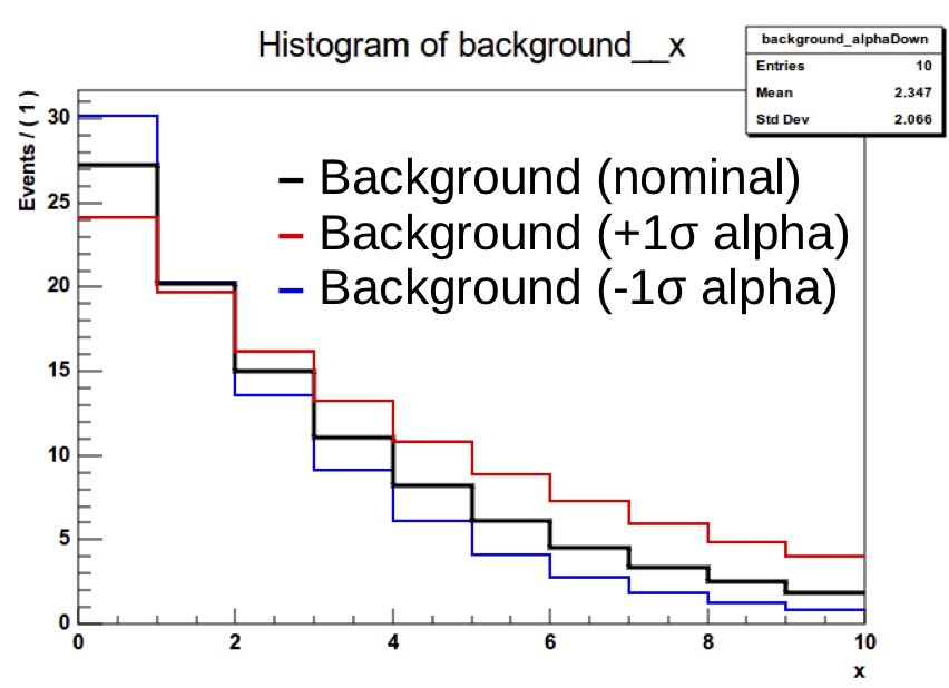
Shape uncertainties can be added by supplying two additional histograms for a process, corresponding to the distribution obtained by shifting that parameter up and down by one standard deviation. These shapes will be interpolated (see the template shape uncertainties section for details) for shifts within \(\pm1\sigma\) and linearly extrapolated beyond. The normalizations are interpolated linearly in log scale just like we do for log-normal uncertainties.
In the list of uncertainties the interpretation of the values for shape lines is a bit different from lnN. The effect can be "-" or 0 for no effect, 1 for normal effect, and possibly something different from 1 to test larger or smaller effects (in that case, the unit Gaussian is scaled by that factor before using it as parameter for the interpolation).
Tasks and questions:
Have a look at datacard_part2.txt: this is currently set up as a one-bin counting experiment, this means only yields are provided.
The first task is to convert this to a shape analysis: the file datacard_part2.shapes.root contains all the necessary histograms, including those for the relevant shape systematic uncertainties. Add the relevant shapes lines to the top of the datacard (after the kmax line) to map the processes to the correct TH1s in this file. Hint: you will need a different line for the signal process, since their naming patterns are different from the background ones.
Compared to the counting experiment we must also consider the effect of uncertainties that change the shape of the distribution. Some, like CMS_eff_t_highpt, are already present in the datacard, as it has both a shape and normalisation effect.
Add the following shape uncertainties: top_pt_ttbar_shape affecting ttbar,the tau energy scale uncertainties CMS_scale_t_1prong0pi0_13TeV, CMS_scale_t_1prong1pi0_13TeV and CMS_scale_t_3prong0pi0_13TeV affecting all processes except jetFakes, and CMS_eff_t_highpt also affecting the same processes.
Once this is done you can convert the text datacard into a RooFit workspace. If we feed the datacard directly into Combine, this step will be done internally every time we run. It is a good idea to do it explicitely especially for more complex analyses, since the conversion step can take a notable amount of time. For this we use the text2workspace.py command:
text2workspace.py datacard_part2.txt -m 800 -o workspace_part2.root
AsymptoticLimits method we can choose just to run the expected limit (--run expected), so as not to calculate the observed. However the data is still used, even for the expected, since in the frequentist approach a background-only fit to the data is performed to define the Asimov dataset used to calculate the expected limits. To skip this fit to data and use the pre-fit state of the model the option --run blind or --noFitAsimov can be used.
A more general way of blinding is to use combine's toy and Asimov dataset generating functionality (--expectSignal [X] -t -1). You can read more about this here. These options can be used with any method in combine, not just AsymptoticLimits.
Now we can finally test our setup:
combine -M AsymptoticLimits workspace_part2.root -m 800 --run blind
Tasks and questions:
- Try to remove (comment out) the shape defining lines and systematics. This effectively transforms our shape analysis into a bin counting one. How much does the sensitivity of the shape analysis improved over the counting analysis?
- Compare the expected limits calculated with --run expected and --run blind. Why are they different?
- You can open the workspace ROOT file interactively and print the contents: w->Print();. Each process is represented by a PDF object that depends on the shape morphing nuisance parameters. From the workspace, choose a process and shape uncertainty, and make a plot overlaying the nominal shape with different values of the shape morphing nuisance parameter. You can change the value of a parameter with w->var("X")->setVal(Y), and access a particular pdf with w->pdf("Z"). PDF objects in RooFit have a createHistogram method that requires the name of the observable (the variable defining the x-axis) - this is called CMS_th1x in combine datacards. Feel free to ask for help with this!
B: MC Statistical uncertainties
On top of yield and shape systematics, there is an important source of uncertainty we should introduce. Our estimates of the backgrounds come either from MC simulation or from sideband regions in data, and in both cases these estimates are subject to a statistical uncertainty on the number of simulated or data events.
In principle we should include an independent statistical uncertainty for every bin of every process in our model.
It's important to note that Combine/RooFit does not take this into account automatically - statistical fluctuations of the data are implicitly accounted for in the likelihood formalism, but statistical uncertainties in the model must be specified by us.
One way to implement these uncertainties is to create a shape uncertainty for each bin of each process, in which the up and down histograms have the contents of the bin
shifted up and down by the \(1\sigma\) uncertainty.
However this makes the likelihood evaluation computationally inefficient, and can lead to a large number of nuisance parameters
in more complex models. Instead we will use a feature in Combine called autoMCStats that creates these automatically from the datacard,
and uses a technique called "Barlow-Beeston-lite" to reduce the number of systematic uncertainties that are created.
This works on the assumption that for high MC event counts we can model the uncertainty with a Gaussian distribution. Given the uncertainties in different bins are independent, the total uncertainty of several processes in a particular bin is just the sum of \(N\) individual Gaussians, which is itself a Gaussian distribution.
So instead of \(N\) nuisance parameters we need only one. This breaks down when the number of events is small and we are not in the Gaussian regime.
The autoMCStats tool has a threshold setting on the number of events below which the the Barlow-Beeston-lite approach is not used, and instead a
Poisson PDF is used to model per-process uncertainties in that bin.
After reading the full documentation on autoMCStats here, add the corresponding line to your datacard.
Start by setting a threshold of 0, i.e. [channel] autoMCStats 0, to force the use of Barlow-Beeston-lite in all bins.
When running the text2workspace step on a datacard with autoMCStats enabled, you will get a report on how each bin has been treated by this algorithm.
Tasks and questions:
- Try to increase the Poisson threshold. How does the text2workspace report changes?
C: Control regions
In a modern analysis it is typical for some or all of the backgrounds to be estimated using the data, instead of relying purely on MC simulation. This can take many forms, but a common approach is to use "control regions" (CRs) that are pure and/or have higher statistics for a given process. These are defined by event selections that are similar to, but non-overlapping with, the signal region. In our \(\phi\rightarrow\tau\tau\) example the \(\text{Z}\rightarrow\tau\tau\) background normalisation can be calibrated using a \(\text{Z}\rightarrow\mu\mu\) CR, and the \(\text{t}\bar{\text{t}}\) background using an \(e+\mu\) CR. By comparing the number of data events in these CRs to our MC expectation we can obtain scale factors to apply to the corresponding backgrounds in the signal region (SR). The idea is that the data will gives us a more accurate prediction of the background with less systematic uncertainties. For example, we can remove the cross section and acceptance uncertainties in the SR, since we are no longer using the MC prediction (with a caveat discussed below). While we could simply derive these correction factors and apply them to our signal region datacard a better way is to include these regions in our fit model and tie the normalisations of the backgrounds in the CR and SR together. This has a number of advantages:
- Automatically handles the statistical uncertainty due to the number of data events in the CR
- Allows for the presence of some signal contamination in the CR to be handled correctly
- The CRs are typically not 100% pure in the background they're meant to control - other backgrounds may be present, with their own systematic uncertainties, some of which may be correlated with the SR or other CRs. Propagating these effects through to the SR "by hand" can become very challenging.
In this section we will continue to use the same SR as in the previous one, however we will switch to a lower signal mass hypothesis, \(m_{\phi}=200\)GeV, as its sensitivity depends more strongly on the background prediction than the high mass signal, so is better for illustrating the use of CRs. Here the nominal signal (r=1) has been normalised to a cross section of 1 pb.
The SR datacard for the 200 GeV signal is datacard_part3.txt. Two further datacards are provided: datacard_part3_ttbar_cr.txt and datacard_part3_DY_cr.txt
which represent the CRs for the Drell-Yan and \(\text{t}\bar{\text{t}}\) processes as described above.
The cross section and acceptance uncertainties for these processes have pre-emptively been removed from the SR card.
However we cannot get away with neglecting acceptance effects altogether.
We are still implicitly using the MC simulation to predict to the ratio of events in the CR and SR, and this ratio will in general carry a theoretical acceptance uncertainty.
If the CRs are well chosen then this uncertainty should be smaller than the direct acceptance uncertainty in the SR however.
The uncertainties acceptance_ttbar_cr and acceptance_DY_cr have been added to these datacards cover this effect. Task: Calculate the ratio of CR to SR events for these two processes, as well as their CR purity to verify that these are useful CRs.
The next step is to combine these datacards into one, which is done with the combineCards.py script:
combineCards.py signal_region=datacard_part3.txt ttbar_cr=datacard_part3_ttbar_cr.txt DY_cr=datacard_part3_DY_cr.txt &> part3_combined.txt
Each argument is of the form [new channel name]=[datacard.txt]. The new datacard is written to the screen by default, so we redirect the output into our new datacard file. The output looks like:
Show datacard
imax 3 number of bins
jmax 8 number of processes minus 1
kmax 15 number of nuisance parameters
----------------------------------------------------------------------------------------------------------------------------------
shapes *              DY_cr          datacard_part3_DY_cr.shapes.root DY_control_region/$PROCESS DY_control_region/$PROCESS_$SYSTEMATIC
shapes *              signal_region  datacard_part3.shapes.root signal_region/$PROCESS signal_region/$PROCESS_$SYSTEMATIC
shapes bbHtautau      signal_region  datacard_part3.shapes.root signal_region/bbHtautau$MASS signal_region/bbHtautau$MASS_$SYSTEMATIC
shapes *              ttbar_cr       datacard_part3_ttbar_cr.shapes.root tt_control_region/$PROCESS tt_control_region/$PROCESS_$SYSTEMATIC
----------------------------------------------------------------------------------------------------------------------------------
bin          signal_region  ttbar_cr       DY_cr
observation  3416           79251          365754
----------------------------------------------------------------------------------------------------------------------------------
bin                                               signal_region  signal_region  signal_region  signal_region  signal_region  ttbar_cr       ttbar_cr       ttbar_cr       ttbar_cr       ttbar_cr       DY_cr          DY_cr          DY_cr          DY_cr          DY_cr          DY_cr
process                                           bbHtautau      ttbar          diboson        Ztautau        jetFakes       W              QCD            ttbar          VV             Ztautau        W              QCD            Zmumu          ttbar          VV             Ztautau
process                                           0              1              2              3              4              5              6              1              7              3              5              6              8              1              7              3
rate                                              198.521        683.017        96.5185        742.649        2048.94        597.336        308.965        67280.4        10589.6        150.025        59.9999        141.725        305423         34341.1        5273.43        115.34
----------------------------------------------------------------------------------------------------------------------------------
CMS_eff_b               lnN                       1.02           1.02           1.02           1.02           -              -              -              -              -              -              -              -              -              -              -              -
CMS_eff_e               lnN                       -              -              -              -              -              1.02           -              -              1.02           1.02           -              -              -              -              -              -
...
The [new channel name]= part of the input arguments is not required, but it gives us control over how the channels in the combined card will be named,
otherwise default values like ch1, ch2 etc will be used.
We now have a combined datacard that we can run text2workspace.py on and start doing fits, however there is still one important ingredient missing. Right now the yields of the Ztautau process in the SR and Zmumu in the CR are not connected to each other in any way, and similarly for the ttbar processes. In the fit both would be adjusted by the nuisance parameters only, and constrained to the nominal yields. To remedy this we introduce rateParam directives to the datacard. A rateParam is a new free parameter that multiples the yield of a given process, just in the same way the signal strength r multiplies the signal yield. The syntax of a rateParam line in the datacard is
[name] rateParam [channel] [process] [init] [min,max]
where name is the chosen name for the parameter, channel and process specify which (channel, process) combination it should affect, init gives the initial value, and optionally [min,max] specifies the ranges on the RooRealVar that will be created. The channel and process arguments support the use of the wildcard * to match multiple entries. Task: Add two rateParams with nominal values of 1.0 to the end of the combined datacard named rate_ttbar and rate_Zll. The former should affect the ttbar process in all channels, and the latter should affect the Ztautau and Zmumu processes in all channels. Set ranges of [0,5] to both. Note that a rateParam name can be repeated to apply it to multiple processes, e.g.:
rateScale rateParam * procA 1.0
rateScale rateParam * procB 1.0
is perfectly valid and only one rateParam will be created. These parameters will allow the yields to float in the fit without prior constraint (unlike a regular lnN or shape systematic), with the yields in the CRs and SR tied together.
Tasks and questions:
- To compare to the previous approach of fitting the SR only, with cross section and acceptance uncertainties restored, an additional card is provided: datacard_part3_nocrs.txt. Run the same fit on this card to verify the improvement of the SR+CR approach
Part 2: Setup Validation
Topics covered in this section:
- A: Using FitDiagnostics to validate your setup
- B: Nuisance parameters impacts
- C: Post-fit distributions
[!TIP] These steps are usually part of the unblinding stage, and are the latest steps request for the GoingToPreApproval. L2 will usually ask to see the results of these procedures before letting you progress further in the review. For most analyses, you will need to first run impact and validation blind, and then repeat it on the actual data.
[!INFO] Analysis datacard must be stored in the CMS analysis GitLab repo GitLab repository. When you request your analysis area, CAT will provide you automatic CI tools that can run all these tests for you every time you commit a change! These are quite flexible and customisable, and you are encouraged to take advantage of them
A: Using FitDiagnostics
Now that we have a working datacard complete with systematic uncertainties, it is important to validate our model. We will explore one of the most commonly used modes of Combine: FitDiagnostics . As well as allowing us to make a measurement of some physical quantity (as opposed to just setting a limit on it), this method is useful to gain additional information about the model and the behaviour of the fit. It performs two fits:
- A "background-only" (b-only) fit: first POI (usually "r") fixed to zero
- A "signal+background" (s+b) fit: all POIs are floating
With the s+b fit Combine will report the best-fit value of our signal strength modifier r. As well as the usual output file, a file named fitDiagnosticsTest.root is produced which contains additional information. In particular it includes two RooFitResult objects, one for the b-only and one for the s+b fit, which store the fitted values of all the nuisance parameters (NPs) and POIs as well as estimates of their uncertainties. The covariance matrix from both fits is also included, from which we can learn about the correlations between parameters. Run the FitDiagnostics method on the workspace we obtained using the SR-only datacard:
combine -M FitDiagnostics workspace_part2.root -m 800 --rMin -20 --rMax 20
fitDiagnosticsTest.root interactively and print the contents of the s+b RooFitResult:
root [1] fit_s->Print()
Show output
RooFitResult: minimized FCN value: -2.55338e-05, estimated distance to minimum: 7.54243e-06
                covariance matrix quality: Full, accurate covariance matrix
                Status : MINIMIZE=0 HESSE=0

    Floating Parameter    FinalValue +/-  Error
  --------------------  --------------------------
             CMS_eff_b   -4.5380e-02 +/-  9.93e-01
             CMS_eff_t   -2.6311e-01 +/-  7.33e-01
      CMS_eff_t_highpt   -4.7146e-01 +/-  9.62e-01
  CMS_scale_t_1prong0pi0_13TeV   -1.5989e-01 +/-  5.93e-01
  CMS_scale_t_1prong1pi0_13TeV   -1.6426e-01 +/-  4.94e-01
  CMS_scale_t_3prong0pi0_13TeV   -3.0698e-01 +/-  6.06e-01
    acceptance_Ztautau   -3.1262e-01 +/-  8.62e-01
        acceptance_bbH   -2.8676e-05 +/-  1.00e+00
      acceptance_ttbar    4.9981e-03 +/-  1.00e+00
            lumi_13TeV   -5.6366e-02 +/-  9.89e-01
         norm_jetFakes   -9.3327e-02 +/-  2.56e-01
                     r   -2.7220e+00 +/-  2.59e+00
    top_pt_ttbar_shape    1.7586e-01 +/-  7.00e-01
          xsec_Ztautau   -1.6007e-01 +/-  9.66e-01
          xsec_diboson    3.9758e-02 +/-  1.00e+00
            xsec_ttbar    5.7794e-02 +/-  9.46e-01
There are several useful pieces of information here. At the top the status codes from the fits that were performed is given. In this case we can see that two algorithms were run: MINIMIZE and HESSE, both of which returned a successful status code (0). Both of these are routines in the Minuit2 minimization package - the default minimizer used in RooFit. The first performs the main fit to the data, and the second calculates the covariance matrix at the best-fit point. It is important to always check this second step was successful and the message "Full, accurate covariance matrix" is printed, otherwise the parameter uncertainties can be very inaccurate, even if the fit itself was successful.
Underneath this the best-fit values (\(\theta\)) and symmetrised uncertainties for all the floating parameters are given. For all the constrained nuisance parameters a convention is used by which the nominal value (\(\theta_I\)) is zero, corresponding to the mean of a Gaussian constraint PDF with width 1.0, such that the parameter values \(\pm 1.0\) correspond to the \(\pm 1\sigma\) input uncertainties.
A more useful way of looking at this is to compare the pre- and post-fit values of the parameters, to see how much the fit to data has shifted and constrained these parameters with respect to the input uncertainty. The script diffNuisances.py can be used for this:
python diffNuisances.py fitDiagnosticsTest.root --all
Show output
name                                              b-only fit            s+b fit         rho
CMS_eff_b                                        -0.04, 0.99        -0.05, 0.99       +0.01
CMS_eff_t                                     * -0.24, 0.73*     * -0.26, 0.73*       +0.06
CMS_eff_t_highpt                              * -0.56, 0.94*     * -0.47, 0.96*       +0.02
CMS_scale_t_1prong0pi0_13TeV                  * -0.17, 0.58*     * -0.16, 0.59*       -0.04
CMS_scale_t_1prong1pi0_13TeV                  ! -0.12, 0.45!     ! -0.16, 0.49!       +0.20
CMS_scale_t_3prong0pi0_13TeV                  * -0.31, 0.61*     * -0.31, 0.61*       +0.02
acceptance_Ztautau                            * -0.31, 0.86*     * -0.31, 0.86*       -0.05
acceptance_bbH                                   +0.00, 1.00        -0.00, 1.00       +0.05
acceptance_ttbar                                 +0.01, 1.00        +0.00, 1.00       +0.00
lumi_13TeV                                       -0.05, 0.99        -0.06, 0.99       +0.01
norm_jetFakes                                 ! -0.09, 0.26!     ! -0.09, 0.26!       -0.05
top_pt_ttbar_shape                            * +0.24, 0.69*     * +0.18, 0.70*       +0.22
xsec_Ztautau                                     -0.16, 0.97        -0.16, 0.97       -0.02
xsec_diboson                                     +0.03, 1.00        +0.04, 1.00       -0.02
xsec_ttbar                                       +0.08, 0.95        +0.06, 0.95       +0.02
The numbers in each column are respectively \(\frac{\theta-\theta_I}{\sigma_I}\) (This is often called the pull, but note that this is a misnomer. In this tutorial we will refer to it as the fitted value of the nuisance parameter relative to the input uncertainty. The true pull is defined as discussed under diffPullAsym here ), where \(\sigma_I\) is the input uncertainty; and the ratio of the post-fit to the pre-fit uncertainty \(\frac{\sigma}{\sigma_I}\).
Tasks and questions:
- Using the SR card, Which parameter has the largest shift from the nominal value (0) in the fitted value of the nuisance parameter relative to the input uncertainty? Which has the tightest constraint?
- Check how much the cross section measurement and uncertainties change using
FitDiagnostics. - It is also useful to check how the expected uncertainty changes using an Asimov dataset, say with
r=10injected. - Should we be concerned when a parameter is more strongly constrained than the input uncertainty (i.e. \(\frac{\sigma}{\sigma_I}<1.0\))?
- Check the fitted values of the nuisance parameters and constraints on a b-only and s+b asimov dataset instead. This check is required for all analyses in the Higgs PAG. It serves both as a closure test (do we fit exactly what signal strength we input?) and a way to check whether there are any infeasibly strong constraints while the analysis is still blind (typical example: something has probably gone wrong if we constrain the luminosity uncertainty to 10% of the input!)
- Run
text2workspace.pyon the combined card (don't forget to set the mass and output name-m 200 -o workspace_part3.root) and then useFitDiagnosticson an Asimov dataset withr=1to get the expected uncertainty. Suggested command line options:--rMin 0 --rMax 2
- Run
- Using the RooFitResult in the
fitDiagnosticsTest.rootfile, check the post-fit value of the rateParams. To what level are the normalisations of the DY and ttbar processes constrained? - Advanced task: Sometimes there are problems in the fit model that aren't apparent from only fitting the Asimov dataset, but will appear when fitting randomised data. Follow the exercise on toy-by-toy diagnostics here to explore the tools available for this.
B: Nuisance parameter impacts
It is often useful to examine in detail the effects the systematic uncertainties have on the signal strength measurement. This is often referred to as calculating the "impact" of each uncertainty. What this means is to determine the shift in the signal strength, with respect to the best-fit, that is induced if a given nuisance parameter is shifted by its \(\pm1\sigma\) post-fit uncertainty values. If the signal strength shifts a lot, it tells us that it has a strong dependency on this systematic uncertainty. In fact, what we are measuring here is strongly related to the correlation coefficient between the signal strength and the nuisance parameter. The MultiDimFit method has an algorithm for calculating the impact for a given systematic: --algo impact -P [parameter name], but it is typical to use a higher-level script, combineTool.py, to automatically run the impacts for all parameters. Full documentation on this is given here. There is a three step process for running this. First we perform an initial fit for the signal strength and its uncertainty:
combineTool.py -M Impacts -d workspace_part3.root -m 200 --rMin -1 --rMax 2 --robustFit 1 --doInitialFit
combineTool.py -M Impacts -d workspace_part3.root -m 200 --rMin -1 --rMax 2 --robustFit 1 --doFits
combineTool.py -M Impacts -d workspace_part3.root -m 200 --rMin -1 --rMax 2 --robustFit 1 --output impacts.json
plotImpacts.py -i impacts.json -o impacts
Tasks and questions:
- Identify the most important uncertainties using the impacts tool.
- In the plot, some parameters do not show a fitted value of the nuisance parameter relative to the input uncertainty, but rather just a numerical value - why?
C: Post-fit distributions
Another thing the FitDiagnostics mode can help us with is visualising the distributions we are fitting, and the uncertainties on those distributions, both before the fit is performed ("pre-fit") and after ("post-fit"). The pre-fit can give us some idea of how well our uncertainties cover any data-MC discrepancy, and the post-fit if discrepancies remain after the fit to data (as well as possibly letting us see the presence of a significant signal!).
To produce these distributions add the --saveShapes and --saveWithUncertainties options when running FitDiagnostics:
combine -M FitDiagnostics workspace_part3.root -m 200 --rMin -1 --rMax 2 --saveShapes --saveWithUncertainties -n .part3B
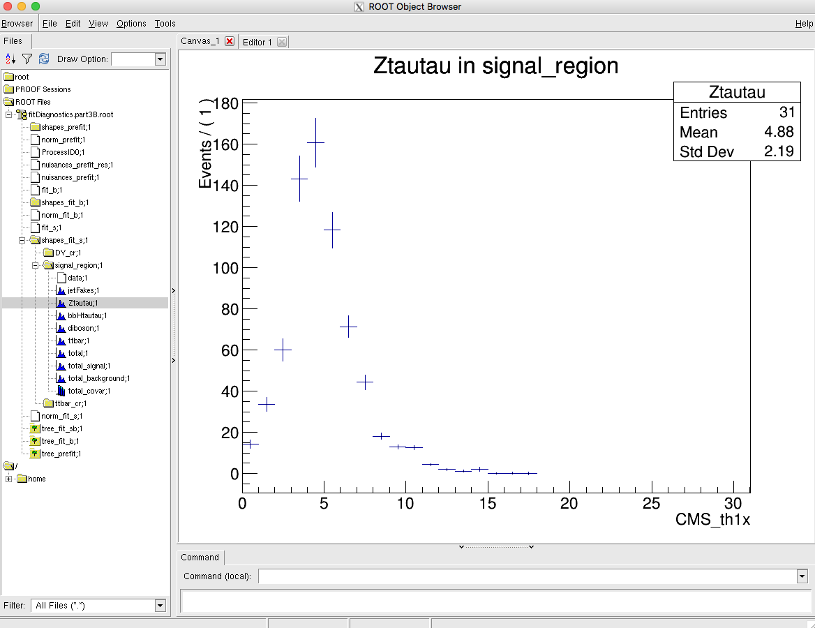
Combine will produce pre- and post-fit distributions (for fit_s and fit_b) in the fitDiagnosticsTest.root output file:
Tasks and questions:
-
Make a plot showing the expected background and signal contributions using the output from
FitDiagnostics- do this for both the pre-fit and post-fit. You will find a scriptpostFitPlot.pyin thedata/tutorials/longexercisedirectory that can help you get started. The bin errors on the TH1s in the fitDiagnostics file are determined from the systematic uncertainties. In the post-fit these take into account the additional constraints on the nuisance parameters as well as any correlations. -
Why is the uncertainty on the post-fit so much smaller than on the pre-fit?
Part 3: Running the fit
Topics covered in this section:
- A: Calculating the significance
- B: Signal strength measurement and uncertainty breakdown
- C: Computing limits with toys
[!TIP] Now you can finally get your final results! The ARC will need to see, check, and comment on your results before they can GL the analysis. While some result can be added to the paper during the ARC review, the main results should be reviewed by L3 and L2 as well and so should be ready by the preapproval talk.
Now that we have a working and validated setup, we can finally perform the statistical analysis of our results. We already saw in the previous sections how to extract limits on our signal under the assumption of the asymptotic regime. Combine provides several other methods to extract different results. In this part we will discuss the most common ones, but you are encouraged to explore the documentation to have a look at the other possibilities offered by the tool.
A: Calculating the significance
In the event that you observe a deviation from your null hypothesis, in this case the b-only hypothesis, Combine can be used to calculate the p-value or significance. To do this using the asymptotic approximation simply do:
combine -M Significance workspace_part3.root -m 200 --rMin -1 --rMax 2
combine -M Significance workspace_part3.root -m 200 --rMin -1 --rMax 5 -t -1 --expectSignal 1.5
--toysFrequentist, which causes a fit to the data to be performed first (with r frozen to the --expectSignal value) and then any subsequent Asimov datasets or toys are generated using the post-fit values of the model parameters. In general this will result in a different value for the expected significance due to changes in the background normalisation and shape induced by the fit to data:
combine -M Significance workspace_part3.root -m 200 --rMin -1 --rMax 5 -t -1 --expectSignal 1.5 --toysFrequentist
Tasks and questions:
- Note how much the expected significance changes with the --toysFrequentist option. Does the change make sense given the difference in the post-fit and pre-fit distributions you looked at in the previous section?
- Advanced task It is also possible to calculate the significance using toys with
HybridNew(details here) if we are in a situation where the asymptotic approximation is not reliable or if we just want to verify the result. Why might this be challenging for a high significance, say larger than \(5\sigma\)?
B: Signal strength measurement and uncertainty breakdown
We have seen that with FitDiagnostics we can make a measurement of the best-fit signal strength and uncertainty. In the asymptotic approximation we find an interval at the \(\alpha\) CL around the best fit by identifying the parameter values at which our test statistic \(q=−2\Delta \ln L\) equals a critical value. This value is the \(\alpha\) quantile of the \(\chi^2\) distribution with one degree of freedom. In the expression for q we calculate the difference in the profile likelihood between some fixed point and the best-fit.
Depending on what we want to do with the measurement, e.g. whether it will be published in a journal, we may want to choose a more precise method for finding these intervals. There are a number of ways that parameter uncertainties are estimated in combine, and some are more precise than others:
- Covariance matrix: calculated by the Minuit HESSE routine, this gives a symmetric uncertainty by definition and is only accurate when the profile likelihood for this parameter is symmetric and parabolic.
- Minos error: calculated by the Minuit MINOS route - performs a search for the upper and lower values of the parameter that give the critical value of \(q\) for the desired CL. Return an asymmetric interval. This is what
FitDiagnosticsdoes by default, but only for the parameter of interest. Usually accurate but prone to fail on more complex models and not easy to control the tolerance for terminating the search. - RobustFit error: a custom implementation in combine similar to Minos that returns an asymmetric interval, but with more control over the precision. Enabled by adding
--robustFit 1when runningFitDiagnostics. - Explicit scan of the profile likelihood on a chosen grid of parameter values. Interpolation between points to find parameter values corresponding to appropriate d. It is a good idea to use this for important measurements since we can see by eye that there are no unexpected features in the shape of the likelihood curve.
In this section we will look at the last approach, using the MultiDimFit mode of combine. By default this mode just performs a single fit to the data:
combine -M MultiDimFit workspace_part3.root -n .part3E -m 200 --rMin -1 --rMax 2
You should see the best-fit value of the signal strength reported and nothing else. By adding the --algo X option combine will run an additional algorithm after this best fit. Here we will use --algo grid, which performs a scan of the likelihood with r fixed to a set of different values. The set of points will be equally spaced between the --rMin and --rMax values, and the number of points is controlled with --points N:
combine -M MultiDimFit workspace_part3.root -n .part3E -m 200 --rMin -1 --rMax 2 --algo grid --points 30
The results of the scan are written into the output file, if opened interactively should see:
Show output
root [1] limit->Scan("r:deltaNLL")
************************************
*    Row   *         r *  deltaNLL *
************************************
*        0 * 0.5399457 *         0 *
*        1 * -0.949999 * 5.6350698 *
*        2 * -0.850000 * 4.9482779 *
*        3 *     -0.75 * 4.2942519 *
*        4 * -0.649999 * 3.6765284 *
*        5 * -0.550000 * 3.0985388 *
*        6 * -0.449999 * 2.5635135 *
*        7 * -0.349999 * 2.0743820 *
*        8 *     -0.25 * 1.6337506 *
*        9 * -0.150000 * 1.2438088 *
*       10 * -0.050000 * 0.9059833 *
*       11 * 0.0500000 * 0.6215767 *
*       12 * 0.1500000 * 0.3910581 *
*       13 *      0.25 * 0.2144184 *
*       14 * 0.3499999 * 0.0911308 *
*       15 * 0.4499999 * 0.0201983 *
*       16 * 0.5500000 * 0.0002447 *
*       17 * 0.6499999 * 0.0294311 *
*       18 *      0.75 * 0.1058298 *
*       19 * 0.8500000 * 0.2272539 *
*       20 * 0.9499999 * 0.3912534 *
*       21 * 1.0499999 * 0.5952836 *
*       22 * 1.1499999 * 0.8371513 *
*       23 *      1.25 * 1.1142146 *
*       24 * 1.3500000 * 1.4240909 *
*       25 * 1.4500000 * 1.7644306 *
*       26 * 1.5499999 * 2.1329684 *
*       27 * 1.6499999 * 2.5273966 *
*       28 *      1.75 * 2.9458723 *
*       29 * 1.8500000 * 3.3863399 *
*       30 * 1.9500000 * 3.8469560 *
************************************
To turn this into a plot run:
python plot1DScan.py higgsCombine.part3E.MultiDimFit.mH200.root -o single_scan
In the next step we will split this total uncertainty into two components. It is typical to separate the contribution from statistics and systematics, and sometimes even split the systematic part into different components. This gives us an idea of which aspects of the uncertainty dominate.
The statistical component is usually defined as the uncertainty we would have if all the systematic uncertainties went to zero. We can emulate this effect by freezing all the nuisance parameters when we do the scan in r,
such that they do not vary in the fit. This is achieved by adding the --freezeParameters allConstrainedNuisances option. It would also work if the parameters are specified explicitly, e.g. --freezeParameters CMS_eff_t,lumi_13TeV,..., but the allConstrainedNuisances option is more concise. Run the scan again with the systematics frozen, and use the plotting script to overlay this curve with the previous one:
combine -M MultiDimFit workspace_part3.root -n .part3E.freezeAll -m 200 --rMin -1 --rMax 2 --algo grid --points 30 --freezeParameters allConstrainedNuisances
python plot1DScan.py higgsCombine.part3E.MultiDimFit.mH200.root --others 'higgsCombine.part3E.freezeAll.MultiDimFit.mH200.root:FreezeAll:2' -o freeze_first_attempt
This doesn't look quite right - the best-fit has been shifted because unfortunately the --freezeParameters option acts before the initial fit, whereas we only want to add it for the scan after this fit. To remedy this we can use a feature of Combine that lets us save a "snapshot" of the best-fit parameter values, and reuse this snapshot in subsequent fits. First we perform a single fit, adding the --saveWorkspace option:
combine -M MultiDimFit workspace_part3.root -n .part3E.snapshot -m 200 --rMin -1 --rMax 2 --saveWorkspace
combine -M MultiDimFit higgsCombine.part3E.snapshot.MultiDimFit.mH200.root -n .part3E.freezeAll -m 200 --rMin -1 --rMax 2 --algo grid --points 30 --freezeParameters allConstrainedNuisances --snapshotName MultiDimFit
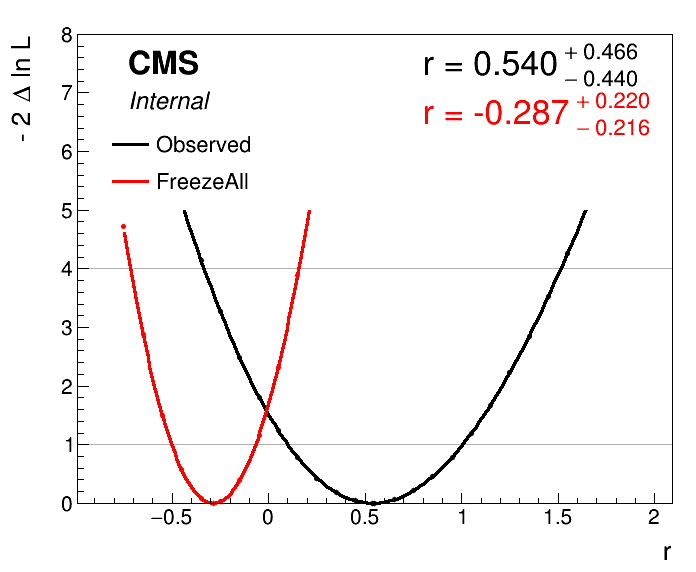
python plot1DScan.py higgsCombine.part3E.MultiDimFit.mH200.root --others 'higgsCombine.part3E.freezeAll.MultiDimFit.mH200.root:FreezeAll:2' -o freeze_second_attempt --breakdown Syst,Stat
Now the plot should look correct:
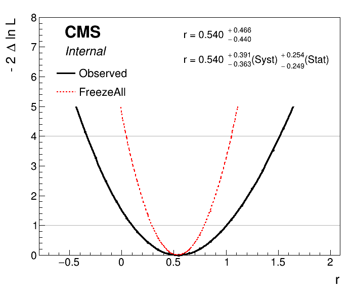
We added the --breakdown Syst,Stat option to the plotting script to make it calculate the systematic component, which is defined simply as \(\sigma_{\text{syst}} = \sqrt{\sigma^2_{\text{tot}} - \sigma^2_{\text{stat}}}\).
To split the systematic uncertainty into different components we just need to run another scan with a subset of the systematics frozen. For example, say we want to split this into experimental and theoretical uncertainties, we would calculate the uncertainties as:
\(\sigma_{\text{theory}} = \sqrt{\sigma^2_{\text{tot}} - \sigma^2_{\text{fr.theory}}}\)
\(\sigma_{\text{expt}} = \sqrt{\sigma^2_{\text{fr.theory}} - \sigma^2_{\text{fr.theory+expt}}}\)
\(\sigma_{\text{stat}} = \sigma_{\text{fr.theory+expt}}\)
where fr.=freeze.
While it is perfectly fine to just list the relevant nuisance parameters in the --freezeParameters argument for the \(\sigma_{\text{fr.theory}}\) scan, a convenient way can be to define a named group of parameters in the text datacard and then freeze all parameters in this group with --freezeNuisanceGroups. The syntax for defining a group is:
[group name] group = uncertainty_1 uncertainty_2 ... uncertainty_N
Tasks and questions:
- Take our stat+syst split one step further and separate the systematic part into two: one part for hadronic tau uncertainties and one for all others.
- Do this by defining a
tauIDgroup in the datacard including the following parameters:CMS_eff_t,CMS_eff_t_highpt, and the threeCMS_scale_t_Xuncertainties. - To plot this and calculate the split via the relations above you can just add further arguments to the
--othersoption in theplot1DScan.pyscript. Each is of the form:'[file]:[label]:[color]'. The--breakdownargument should also be extended to three terms. - How important are these tau-related uncertainties compared to the others?
C: Computing limits with toys
Now we will look at computing limits without the asymptotic approximation, so instead using toy datasets to determine the test statistic distributions under the signal+background and background-only hypotheses. This can be necessary if we are searching for signal in bins with a small number of events expected. In Combine we will use the HybridNew method to calculate limits using toys. This mode is capable of calculating limits with several different test statistics and with fine-grained control over how the toy datasets are generated internally. To calculate LHC-style profile likelihood limits (i.e. the same as we did with the asymptotic) we set the option --LHCmode LHC-limits. You can read more about the different options in the Combine documentation.
Run the following command:
combine -M HybridNew datacard_part1.txt --LHCmode LHC-limits -n .part1B --saveHybridResult
AsymptoticLimits this will only determine the observed limit, and will take a few minutes. There will not be much output to the screen while combine is running. You can add the option -v 1 to get a better idea of what is going on. You should see Combine stepping around in r, trying to find the value for which CLs = 0.05, i.e. the 95% CL limit. The --saveHybridResult option will cause the test statistic distributions that are generated at each tested value of r to be saved in the output ROOT file.
To get an expected limit add the option --expectedFromGrid X, where X is the desired quantile, e.g. for the median:
combine -M HybridNew datacard_part1.txt --LHCmode LHC-limits -n .part1B --saveHybridResult --expectedFromGrid 0.500
Calculate the median expected limit and the 68% range. The 95% range could also be done, but note it will take much longer to run the 0.025 quantile. While Combine is running you can move on to the next steps below.
Tasks and questions:
- In contrast to
AsymptoticLimits, withHybridNeweach limit comes with an uncertainty. What is the origin of this uncertainty? - How good is the agreement between the asymptotic and toy-based methods?
- Why does it take longer to calculate the lower expected quantiles (e.g. 0.025, 0.16)? Think about how the statistical uncertainty on the CLs value depends on Pmu and Pb.
Next plot the test statistic distributions stored in the output file:
python3 $CMSSW_BASE/src/HiggsAnalysis/CombinedLimit/test/plotTestStatCLs.py --input higgsCombine.part1B.HybridNew.mH120.root --poi r --val all --mass 120
This produces a new ROOT file test_stat_distributions.root containing the plots, to save them as pdf/png files run this small script and look at the resulting figures:
python3 printTestStatPlots.py test_stat_distributions.root